The Bottleneck
Geometric deep learning models work with data that does not fit a regular grid: point clouds, particle-detector measurements, and other collections of objects with spatial relationships. A nearest-neighbor graph gives these models a local structure to learn from, connecting each point to the points closest to it in feature space.
In dynamic graph networks such as GravNet, those features change as the model learns, so neighborhoods are rebuilt during each forward pass. Graph construction is a recurring computational cost. Exact brute-force k-nearest-neighbor search checks every candidate pair, and that work grows quadratically with the number of points.
FastGraph accelerates this step by organizing points into spatial bins and skipping regions that cannot contain a closer neighbor. The challenge is making that search efficient as the feature space grows, while retaining exact neighbors and fitting into a GPU-based learning pipeline.
The Engineering
Adapt the search to the data. Binning along a few original coordinates can work well when those axes capture useful structure. When they do not, the search may still have to check many candidates. The PCA extension estimates an orthonormal basis from a sample of points on the GPU, then projects the data into a compact search space. The evaluated HGCAL configuration uses three binning dimensions for eight-dimensional inputs.
Keep the distance metric intact. The projection organizes the search; neighbor distances are calculated using all of the original features. Points are grouped and sorted into bins, and the search traverses expanding shells around each query while maintaining its closest neighbors. Separate graphs are kept apart through row splits, so points from different graphs cannot become neighbors.
Skip candidates with a valid bound. An orthonormal projection cannot increase Euclidean distance. This makes the distance to an unvisited projected bin a lower bound on the distance to its points in the original space. Once the bound for every unvisited bin exceeds the farthest selected neighbor’s distance, the search can stop. The pruning rule preserves exact neighbors in exact arithmetic; floating-point behavior was checked against brute-force references across multiple dimensions and neighborhood sizes.
Specialize the CUDA implementation. The binning kernels specialize on 2–5 dimensions at compile time, enabling fixed-size storage and loop unrolling. Keeping the binning space small limits grid and traversal costs even when the input has more features. This combines an algorithmic reduction in candidate checks with kernels tailored to the supported search configurations.
Connect the kernels to PyTorch. C++ operator registration and autograd support let the graph-building operations participate in a learning pipeline. Gradients propagate through selected distances and input coordinates, while discrete neighbor indices remain fixed for each forward/backward pair. The axis-aligned path also supports TorchScript; the PCA wrapper runs in eager mode.
My Role
I developed the PCA-based search extension, rewrote and optimized selected CUDA kernels, and rewrote the paper from the ground up as first author. This work builds on Jan Kieseler’s original kernels and early manuscript.
- Algorithm development. Developed the compact, data-adaptive search extension and its use of projected bounds with full-dimensional distance calculations.
- GPU performance engineering. Reworked selected kernels around compile-time specialization and optimized their performance across the supported binning dimensions.
- Framework integration. Worked on C++ operator registration, autograd, and TorchScript support for the axis-aligned path, with changes merged upstream.
- Paper and analysis. Rebuilt the manuscript’s method explanation, exactness argument, experimental analysis, and discussion of where the approach performs well and where it does not.
Performance
On the evaluated CMS HGCAL detector-derived workload, the PCA implementation reports a 41.23× speedup over exact FAISS-GPU and a 19.41× speedup over cuVS brute force.
That comparison uses 5 million points, 8 features, and 40 neighbors per point in a single graph segment on one NVIDIA A100 80 GB PCIe GPU, with FP32 coordinates, CUDA 12.1, and PyTorch 2.5. Each exact method solves the same nearest-neighbor task.
| Exact method | Graph construction time |
|---|---|
| FastGraph with PCA | 7.5 s |
| cuVS brute force | 146 s |
| FAISS-GPU IndexFlatL2 | 310 s |
Times are rounded medians of seven repetitions; speedups use the unrounded medians. The timed region includes PCA estimation, projection, bin construction, and search, with inputs already on the GPU. Data transfer and downstream training are outside that measurement.
Across the evaluated 2–10-dimensional HGCAL workloads at 5 million points and 40 neighbors, the reported geometric-mean speedup over FAISS-GPU is 10.4×. The figure below shows how performance changes across those configurations.
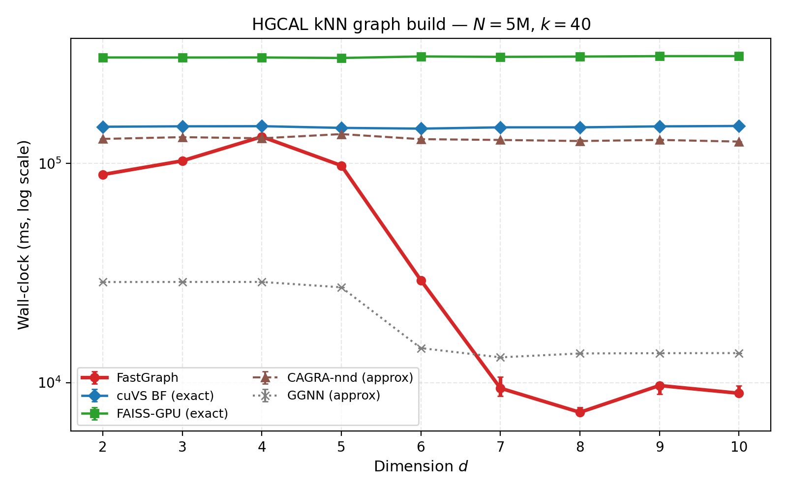 Results from the PCA manuscript. Lower is better; the time axis is logarithmic. GGNN and CAGRA are approximate methods and were not compared at matched recall.
Engineering Tradeoffs
Data geometry determines how much work can be skipped. PCA is useful when a compact subspace captures structure that makes pruning effective. On isotropic data, there may be little useful structure to exploit, and optimized brute force can be faster.
A more elaborate index has its own cost. PCA fitting and projection add overhead, especially for small graphs. Increasing the number of binning dimensions can make the search more selective, but also increases grid size and traversal work. The three-dimensional configuration reflects that balance for the evaluated workload.
The benchmark measures a single-GPU graph-construction operation. Its practical value in a larger model depends on how much of that model’s runtime is spent rebuilding neighborhoods, as well as the size and geometry of its graphs.